by Loren Cobb
This essay is written for any members of the Mechanical Investing community who would like to gain a better understanding of volatility, and for any other investors who may stumble across it while browsing the web. The subject matter is quite technical, but in the interest of intelligibility I have forced myself to avoid the use of equations as much as possible. All comments, corrections, and criticisms will be welcome!
Readers who prefer a more mathematical treatment are referred to The Mathematics of Volatility for details.
In essence, volatility is a measure of the uncertainty of an investment. Every price movement of an investment can be broken down into two parts: one part is the movement we expected, and the other is what we did not expect. Volatility comes from the latter part. In practical terms, volatility is concerned with the difference between observed and expected price movements.
|
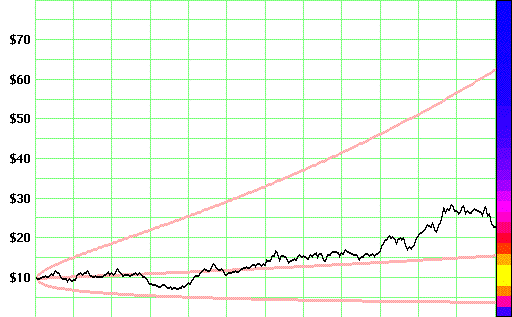
The expected (non-volatile) part of the movement in price of an investment is usually described in terms of an expected growth rate. Over the short term, most investors predict future growth rates from the pattern of recently observed price growth. The ordinary measure used for describing a growth rate is the "compound annualized growth rate", or CAGR. In Figure 1, the central pale red line shows the predicted price growth in an investment that was purchased for $10 and held for twelve months.
The unexpected (volatile) part of the movement in price of an investment is its volatility. This part can go up or down, with equal likelihood, because it is by definition the part that is unpredictable. Due to our uncertainty about price movement, there is a probability distribution of prices, centered on the predicted price. This probability distribution lies at the core of the concept of "volatility." By describing its shape and size, we describe volatility itself. In Figure 1, the probability of each final price is indicated with colors. The color scale runs from blue (least likely) through magenta and red to yellow (most likely).
The colored histogram shown in Figure 1 is based on 25,000 independent runs of a simulated investment whose annual growth rate is 100%, with very high volatility. The effect of the high volatility is very clear in this figure: some investors may easily see a return in excess of 600%, while others may lose over 60%. Consequently, their initial uncertainty as to the outcome of their investments is very large indeed.
 |
Volatility has no traditional or universal measure, but in the Mechanical Investing community we customarily use a measure known as the "geometric standard deviation," or GSD. Elsewhere in the financial analysis literature a closely related measure is used, sigma = ln(1 + GSD/100). These two measures of volatility only make sense in the context of a certain widely-accepted theory of how investment prices change over time. This theory, which for lack of a better term might be called the "geometric Brownian motion model," is in general agreement with a great variety of data. Somewhat better accuracy can be obtained with technical refinements such as the GARCH models, but as a basic theory this model has achieved almost canonical status within the domain of financial analysis.
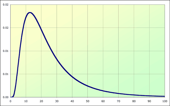
In brief, the principal prediction of the geometric Brownian motion model of investment price movements is that the probability distribution of price movements will have a very particular shape known as the "lognormal" distribution. The GSD is an excellent measure of volatility when the price distribution is roughly lognormal, because it is based on the fundamental parameters of that distribution. In effect, it is just the standard deviation of the logarithms of all investment returns.
Most people, including most investors, find it quite difficult to visualize correctly just how volatility will affect an investment. For this reason, I have constructed a little computer program that can be used as a tutorial laboratory to help inform and guide the intuition with respect to volatility. To download it from my website, click on one of these links: Windows version or Macintosh version. I wrote this "Volatility Laboratory" in order to help myself understand how volatility works, and it has been a great help. In the discussion that follows, almost all of the examples will refer to displays from this lab.
The volatility displayed in Figure 1 is highly asymmetrical. The pale red envelope encloses the region in which the price trajectory is most likely to move; this region clearly expands much more rapidly in the direction of higher prices than it does towards lower. This region is known as the "2-sigma" envelope.
If we transform all prices by taking their logarithms and then replot the graph, then three remarkable things happen:
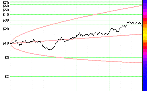 |
This is shown in Figure 3. Notice that the 2-sigma envelope now looks like a quadratic curve laid on its side and skewed upwards so that its central axis lines up with the predicted price line for the investment. This is the origin of the intuition that says that "uncertainty increases like the square-root of time." If you compare the size of the uncertainty to the gain in the predicted price of the stock, it becomes clear that the longer a stock is held the better the price appreciation in comparison to the increase in uncertainty. This is the basis for the "long term buy and hold" strategy, which works well as long as the price of an investment continues to move with the predicted dynamics.
At the very beginning, the volatility increases very rapidly indeed, literally exploding off the initial price point with infinite velocity, then steadily decelerating for the entire duration of the graph.
The GSD of the price trajectory in these two figures was set at 100, which is a very high level of volatility. The CAGR was also set to 100, implying that the investment was expected to double every year. But if you look carefully, you will see that the central red line in the figure does not end at $20, as ordinary intuition might lead you to think it should. Instead, it terminates at $15.74, an amount that is substantially less than the 100% growth rate would seem to imply. Why this occurs is perhaps the single most important point in this essay. This point was first made on the Mechanical Investing board by BarryDTO in post #84987.
If you run a large number of independent simulations of this investment model with parameters held constant, then the average of all final prices is indeed exactly the amount predicted by the growth rate. In the above example, this average is $20, due to 100% appreciation over a period of one year. The probability distribution of prices is highly skewed, however, so the median final price will be much less than the mean. (Recall the definition of the median: 50% of all prices will be higher than the median, and 50% will be lower.) The central pale red line in both figures traces the movement of the median price, not the mean price, over time. Most importantly, the normal distribution that is visible when graphed in logarithmic coordinates is centered on the median price, not the mean price. Thus when the GSD is high, as it is with many speculative investments and high-flying mechanical screens, then the median return that investors will receive is much smaller than the expected or average return. In fact, the entire 2-sigma envelope is much lower than the mean, because it is centered on the median.
To calculate the median price appreciation, one must deflate the CAGR by a fraction that depends on the square of the volatility. A recipe for this calculation is shown in the sidebar to the right.
For example, when CAGR = GSD = 100 the deflator works out to 0.786. Thus the median CAGR is only 1.57, or 57 in percentage terms. |
The result is the median price appreciation. In the example, the effect of a high GSD of 100 was to deflate the CAGR all the way from 100 down to 57. Lower volatilities will cause much less deflation. A volatility of 30, typical of many mechanical screens, implies a deflator of 0.966, meaning that the median return is only 3.4% lower than the mean.
I think it is reasonable to conclude that we need concern ourselves with deflating the CAGR only when the volatility of an investment climbs above 30, or when comparing two investments with similar growth rates but greatly differing levels of volatility. In the latter case, the deflator may actually change the direction of the comparison.
Several further warnings are in order here:
When the market executes a sharp and unexpected move, one often hears heartfelt comments like this, "I hate volatility to the downside, but upside volatility is just fine with me!"
Such comments reveal profound confusion about the very nature of volatility. Although a single movement may go upwards or downwards, by definition volatility is neither upside nor downside. Volatility is not a characteristic of any single movement. Quite the contrary: it is a characteristic of all movements, considered as a single population. This is clear from the way it is measured, based on a standard deviation. As such it describes the size of the typical deviation of the return from its predicted level. These deviations are necessarily equally likely in the positive and negative directions.
Of course, it is always possible to calculate a standard deviation on downward price movements alone, and this has from time to time been proposed as a measure of "downside volatility." Part of the rationale for this measure is the idea that one would like to find an investment whose "upside volatility" is much larger than its "downside volatility." In practice this has not proven useful, almost certainly because the logarithm transformation renders the two kinds of volatility effectively identical, as predicted by the theory of geometric Brownian motion. This is not to say that the two will always be identical for every kind of investment! Instead, the claim is that any investment which conforms roughly to geometric Brownian motion will not benefit from this treatment. Since most investment vehicles do conform, more or less, the effort to define separate meaures for "upside" and "downside" volatility is usually futile.
Risk is defined as the possibility of an unpleasant event. In many investment cases, volatility can be used to calculate lower bounds for the probabilities of these events. For example, many risk-averse investors want to see an explicit calculation of the probability that a particular investment may fall to, say, one-half its initial value. Given believable estimates for the CAGR and GSD of the investment, one can indeed calculate this risk. However, because of the problems identified above in the section entitled "Hidden Assumptions," any such calculation will only give a lower bound — the actual probability is likely to be larger than the calculated value. Still, estimating these kinds of risks is an important component of effective risk management.
For most unpleasant events that can be unambiguously described in terms of the price of an investment, Figure 2 offers a hint of the way in which the risk probabilities are calculated. Since the probability distribution of returns, measured on a logarithmic scale, is the familiar normal bell-shaped curve, one can look up the probability in a table of the normal distribution. In effect this is what is done, though computer methods usually replace the table look-up with a numerical evaluation of the incomplete Gaussian integral.
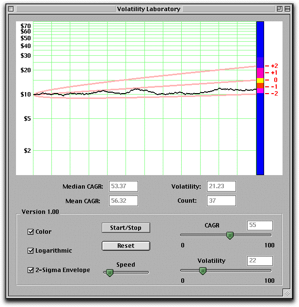 |
For ordinary mortals without access to advanced numerical methods, the Volatility Laboratory offers some help. The display shows the 2-sigma envelope, as it changes in response to changes in the CAGR and Volatility of the investment. Price movements that run outside the 2-sigma envelope occur about 5% of the time, so the probability of dropping below the 2-sigma line is 2.5%. This line provides a point of known risk, allowing one to get a feeling for the probabilities of similar risks.
The CAGR and Volatility of the investment are adjusted with sliders, as shown in the screen shot to the right (Figure 3). The display shows that for an investment with a CAGR of 55, such as the TREPPE screen, the GSD must be 22 in order for the bottom of the 2-sigma envelope to touch the $10 point. In other words, if the volatility exceeds 22 for this screen (which it does — the volatility is about 26), then the probability of a loss after a hold of one year is greater than 2.5%.
The checkbox named "Logarithmic" will change the display instantly between rectilinear and logarithmic styles. For those who see grayscale more accurately than color, there is also a checkbox named "Color" that will switch between colors and grays.
The "Start/Stop" button will start or stop generating simulations of the specified investment process. The final points of these simulations are counted in the histogram depicted on the right-hand side. The display can be shifted between rectilinear and logarithmic without damaging these counts (because counts for two separate histograms are being accumulated, though only one is displayed). The "Speed" slider controls the speed of the simulations.
When simulations are running, three statistics are continuously updated to show current results. Volatility is estimated from the standard deviation of final log returns. This point needs to be emphasized: the displayed volatility statistic is not calculated based on all price movements in a single trajectory, as it is normally down when backtesting an investment strategy. Instead it is calculated from all final returns in the entire population of simulations. Similarly, the mean CAGR is estimated from final returns, and the median from the average of all final log returns. Therefore, these statistics provide a rigorous test of the accuracy of the simulation.
The sliders of the Volatility Laboratory are currently suffering from some unknown programming glitch, visible only in the Windows version, which leaves "ghosts" of the slider on the screen as it is moved. Someday I will figure out how to exorcise these ghosts. Fortunately, they are harmless.
The effort of getting the simulation to work properly turned out to be an education in the construction of random numbers. The first draft of the simulation code yielded volatilities that were 40% lower than theory predicted. Since I had total confidence in the theory and great confidence in my programming skills, the only possible culprit was the random number generator. I had been using a very common method for generating normally-distributed random numbers, in which one simply adds 12 independent uniformly-distributed numbers and subtracts 6. It turns out that this method generates way too few extreme events! So I switched to the Box-Muller algorithm, which is slower but more accurate. This yielded empirical volatilities that were still 5% too low. After much head-scratching and searching through dead-ends, I discovered that the linear congruential algorithm with which almost all computers generate uniform random numbers is deficient — seriously, desperately deficient. Friends, this may not be news to some, but for me it was a revelation. Only after laboriously encoding a three-generator algorithm did I get acceptable agreement between theory and practice. One generator produces the high-order bits of the result, the second produces the low-order bits, and the third shuffles the sequence of output numbers to remove periodicities (this algorithm may be found in Numerical Recipes in C by William Press et al).
I also learned quite a lot about the nitty-gritty details of stochastic differential equations, which is the mathematical basis for the theory of geometric Brownian motion. Now in principle I should have known all this stuff, having used this theory in various contexts throughout my professional career, but when it came down to making a simulation work, not just more or less right but exactly right, I discovered that there were important details with which I had never come to terms. I have written down all of this theory in a second essay, The Mathematics of Volatility so that any who wish to follow the details may do so.
Loren Cobb.
Many thanks to William Lipp and Tim O'Beirne for commenting on an early draft of this essay and its companion software. Any errors that remain are my responsibility, not theirs. Comments and suggestions are always welcome!
The first draft of this essay was completed on 15 May 2002. It was last revised on 17 July 2003.